Scikit-Learn offers several linear models, as mentioned below.
- Linear Regression: This model analyzes the relationship between a dependent variable (i.e., target) and multiple independent variables (i.e., data).
- Logistic Regression: This model is a classification algorithm that estimates discrete values (0 or 1, yes/no, true/false) based on independent variables.
- Ridge Regression: This model adds L2 regularization to the loss function, incorporating a penalty equal to the square of coefficients’ magnitude.
- Bayesian Ridge Regression: This model uses probability distributions for linear regression to handle insufficient or poorly distributed data.
- LASSO: This model applies L1 regularization by adding a penalty based on the absolute values of coefficients to the loss function.
- Multi-task LASSO: This model fits multiple regression problems jointly, enforcing consistent feature selection across tasks, and uses a mixed L1, L2-norm for regularization to estimate sparse coefficients.
- Elastic-Net: This model combines L1 and L2 penalties from Lasso and Ridge regression, effectively handling multiple correlated features.
- Multi-task Elastic-Net: This model fits multiple regression problems simultaneously, enforcing consistent feature selection across all tasks.
The following example shows how to use linear regression for the modeling process based on the Real Estate Data Chicago dataset, using only one of the features, and the results exhibit some characteristics, such as the mean squared error.
import pandas as pd
from sklearn.model_selection import train_test_split
from sklearn.preprocessing import StandardScaler
from sklearn.linear_model import LinearRegression
from sklearn.metrics import mean_squared_error, r2_score
import matplotlib.pyplot as plt
import seaborn as sns

dataset = pd.read_csv('real_estate.csv', usecols = ['sqft', 'listPrice'])
dataset = dataset.dropna()

data_train, data_test, target_train, target_test = train_test_split(dataset[['sqft']], dataset[['listPrice']], test_size = 0.2, random_state = 0)

scaler = StandardScaler()
scaled_data_train = scaler.fit_transform(data_train)
scaled_data_test = scaler.transform(data_test)

model = LinearRegression()
model.fit(scaled_data_train, target_train)
target_pred = model.predict(scaled_data_test)

# Print the results
r2 = r2_score(target_test, target_pred)
print(f"R-squared: {r2:.2f}")
mse = mean_squared_error(target_test, target_pred)
print(f"Mean squared error: {mse:.2f}")
rmse = mse ** 0.5
print(f"Root mean squared error: {rmse:.2f}")

corr_matrix = dataset.corr()
high_corr_features = [(col1, col2, corr_matrix.loc[col1, col2])
                     for col1 in corr_matrix.columns
                     for col2 in corr_matrix.columns
                     if col1 != col2 and abs(corr_matrix.loc[col1, col2]) > 0.8]
collinearity = pd.DataFrame(high_corr_features, columns = ["Feature 1", "Feature 2", "Correlation"])
print("\nHighly correlated features:\n", collinearity)

print("\nIntercept:", model.intercept_)

print("\nFeature coefficients:\n", model.coef_)

# Show the plots
plt.figure(figsize = (12, 5))
residuals = target_test - target_pred

plt.subplot(1, 2, 1)
sns.histplot(residuals, bins = 100, kde = True, color = "blue")
plt.axvline(x = 0, color = 'red', linestyle = '--')
plt.title("Residuals Distribution")
plt.xlabel("Residuals (Actual Price - Predicted Price)")
plt.ylabel("Frequency")

plt.subplot(1, 2, 2)
sns.scatterplot(x = target_test.squeeze(), y = target_pred.squeeze(), alpha = 0.5)
plt.plot([min(target_test.squeeze()), max(target_test.squeeze())], [min(target_test.squeeze()), max(target_test.squeeze())], color = 'red', linestyle = '--')
plt.title("Regression Fit (Actual vs Predicted)")
plt.xlabel("Actual Price")
plt.ylabel("Predicted Price")

plt.tight_layout()
plt.savefig("output")
Output
R-squared: 0.67
Mean squared error: 661765353689.33
Root mean squared error: 813489.61

Highly correlated features:
    Feature 1  Feature 2  Correlation
0       sqft  listPrice     0.823902
1  listPrice       sqft     0.823902

Intercept: [654489.61904762]

Feature coefficients:
 [[1109793.51720412]]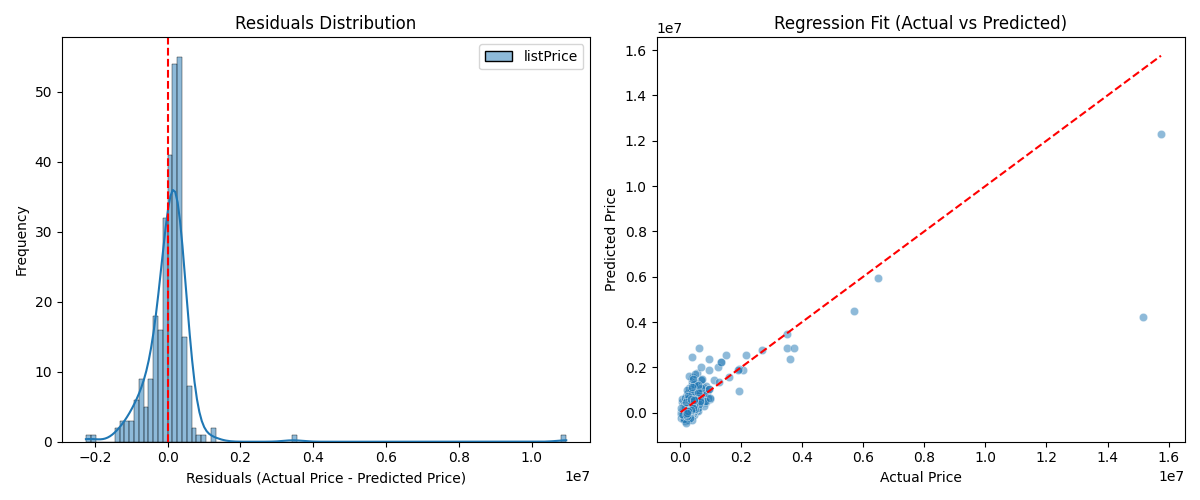
The Real Estate Data Chicago dataset (‘real_estate.csv’) can be download via the link below:
https://www.kaggle.com/datasets/kanchana1990/real-estate-data-chicago-2024The example below illustrates how to apply multiple linear regression for the modeling process based on the same dataset, using two of the features, and the results display some characteristics, such as the root mean squared error.
import pandas as pd
from sklearn.model_selection import train_test_split
from sklearn.preprocessing import StandardScaler
from sklearn.linear_model import LinearRegression
from sklearn.metrics import mean_squared_error, r2_score
import matplotlib.pyplot as plt
import seaborn as sns

dataset = pd.read_csv('real_estate.csv', usecols = ['sqft', 'stories', 'listPrice'])
dataset = dataset.dropna()

data_train, data_test, target_train, target_test = train_test_split(dataset[['sqft', 'stories']], dataset[['listPrice']], test_size = 0.2, random_state = 0)

scaler = StandardScaler()
scaled_data_train = scaler.fit_transform(data_train)
scaled_data_test = scaler.transform(data_test)

model = LinearRegression()
model.fit(scaled_data_train, target_train)
target_pred = model.predict(scaled_data_test)

# Print the results
r2 = r2_score(target_test, target_pred)
print(f"R-squared: {r2:.2f}")
mse = mean_squared_error(target_test, target_pred)
print(f"Mean squared error: {mse:.2f}")
rmse = mse ** 0.5
print(f"Root mean squared error: {rmse:.2f}")

corr_matrix = dataset.corr()
high_corr_features = [(col1, col2, corr_matrix.loc[col1, col2])
                     for col1 in corr_matrix.columns
                     for col2 in corr_matrix.columns
                     if col1 != col2 and abs(corr_matrix.loc[col1, col2]) > 0.8]
collinearity = pd.DataFrame(high_corr_features, columns = ["Feature 1", "Feature 2", "Correlation"])
print("\nHighly correlated features:\n", collinearity)

print("\nIntercept:", model.intercept_)

print("\nFeature coefficients:\n", model.coef_)

# Show the plots
plt.figure(figsize = (12, 5))
residuals = target_test - target_pred

plt.subplot(1, 2, 1)
sns.histplot(residuals, bins = 100, kde = True, color = "blue")
plt.axvline(x = 0, color = 'red', linestyle = '--')
plt.title("Residuals Distribution")
plt.xlabel("Residuals (Actual Price - Predicted Price)")
plt.ylabel("Frequency")

plt.subplot(1, 2, 2)
sns.scatterplot(x = target_test.squeeze(), y = target_pred.squeeze(), alpha = 0.5)
plt.plot([min(target_test.squeeze()), max(target_test.squeeze())], [min(target_test.squeeze()), max(target_test.squeeze())], color = 'red', linestyle = '--')
plt.title("Regression Fit (Actual vs Predicted)")
plt.xlabel("Actual Price")
plt.ylabel("Predicted Price")

plt.tight_layout()
plt.savefig("output")
Output
R-squared: 0.76
Mean squared error: 853564656404.50
Root mean squared error: 923885.63

Highly correlated features:
    Feature 1  Feature 2  Correlation
0       sqft  listPrice     0.823992
1  listPrice       sqft     0.823992

Intercept: [571217.84386973]

Feature coefficients:
 [[876702.02041909 205742.58176765]]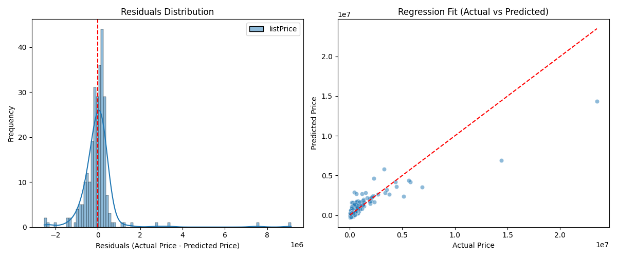
Furthermore, the following example shows how to use logistic regression for linear modeling based on the the Pima-Indian dataset, evaluating this modeling through the confusion matrix and classification report.
from pandas import read_csv
from sklearn.model_selection import train_test_split
from sklearn.linear_model import LogisticRegression
from sklearn import metrics
from sklearn.metrics import classification_report

path = "pima-indians-diabetes.csv"
headers = ['preg', 'plas', 'pres', 'skin', 'test', 'mass', 'pedi', 'age', 'class']
dataset = read_csv(path, names = headers)
data = dataset.values[1:, 0:8]
target = dataset.values[1:, 8]
data_train, data_test, target_train, target_test = train_test_split(data, target, test_size = 0.20, random_state = 0)

regressor = LogisticRegression(penalty = 'l2', C = 2.0, solver = 'liblinear', max_iter = 1000)
regressor.fit(data_train, target_train)
target_prediction = regressor.predict(data_test)

result = metrics.confusion_matrix(target_test, target_prediction)
print("The confusion matrix is:\n", result)

target_names = ["without diabetes", "with diabetes"]
print("\nThe classification report is:")
print(classification_report(target_test, target_prediction, target_names = target_names))
Output
The confusion matrix is:
 [[98  9]
 [19 28]]

The classification report is:
                  precision    recall  f1-score   support

without diabetes       0.84      0.92      0.88       107
   with diabetes       0.76      0.60      0.67        47

        accuracy                           0.82       154
       macro avg       0.80      0.76      0.77       154
    weighted avg       0.81      0.82      0.81       154
The “pima-indians-diabetes.csv” dataset can be downloaded using the following link:
https://github.com/npradaschnor/Pima-Indians-Diabetes-Dataset/blob/master/diabetes.csvReferences
- Hackeling, G. (2017). Mastering Machine Learning with scikit-learn, 2nd Edition. Packt Publishing Ltd.
- Géron, A. (2019). Hands-On Machine Learning with Scikit-Learn, Keras, and TensorFlow, 2nd Edition. O’Reilly Media, Inc.
- Tutorials Point. Scikit Learn Tutorial. Retrieved November 20, 2025, from https://www.tutorialspoint.com/.
Leave a Reply