AysamByte

Clustering methods in Scikit-Learn are essential for identifying similarities among data samples. As a key unsupervised machine learning technique, they reveal patterns and group similar samples based on features, helping to determine intrinsic groupings within unlabeled data, thus emphasizing their importance in data analysis. This library provides the following clustering methods:

• K-Means: This algorithm computes optimal centroids by clustering data into K groups of equal variances, minimizing the inertia criterion. It requires prior knowledge of the number of clusters, iterating until the centroids stabilize to effectively separate samples into designated clusters.
• Affinity Propagation: This algorithm relies on message passing between sample pairs to achieve convergence, requires no pre-specified cluster numbers, but has a time complexity of O(2), its major drawback.
• Mean Shift: This algorithm identifies blobs in smooth density samples, iteratively assigning datapoints to clusters by shifting towards high-density areas, automatically determining the number of clusters instead of relying on a bandwidth parameter.
• Spectral Clustering: This algorithm utilizes eigenvalues from the similarity matrix for dimensionality reduction but is unsuitable for large cluster counts during clustering.
• Hierarchical Clustering: This algorithm constructs nested clusters through successive merging or splitting, represented as a dendrogram. It consists of two categories: agglomerative hierarchical algorithms, where each data point starts as a single cluster and merges pairs in a bottom-up approach; and divisive hierarchical algorithms, which treat all data points as one cluster, splitting it into smaller clusters in a top-down manner.
• DBSCAN: Density-based spatial clustering of applications with noise (DBSCAN) identifies clusters as dense regions within lower-density areas. Scikit-Learn’s module implements this algorithm, relying on two key parameters: min_samples and eps. Adjusting these parameters influences cluster density, where higher min_samples or lower eps indicates a more concentrated distribution of data points required for cluster formation.
• OPTICS: Ordering points to identify the clustering structure (OPTICS) identifies density-based clusters in spatial data, improving on DBSCAN by addressing varying density issues. It orders data points to ensure that spatially closest points are neighbors in the ordering, enhancing cluster detection.
• BIRCH: Balanced iterative reducing and clustering using hierarchies (BIRCH) performs hierarchical clustering on large datasets. It constructs a Characteristics Feature Tree (CFT), where CF nodes contain essential clustering information, reducing memory needs by eliminating the requirement to store the entire input data.

The following example applies the K-Means clustering method to the digits dataset. This algorithm identifies similar digits without using the original label information.

from sklearn.datasets import load_digits
from sklearn.cluster import KMeans
import matplotlib.pyplot as plt
import numpy as np
from scipy.stats import mode
from sklearn.metrics import accuracy_score

dataset = load_digits()
print(dataset.data.shape)

kmeans = KMeans(n_clusters = 10, random_state = 0)
clusters = kmeans.fit_predict(dataset.data)
print(kmeans.cluster_centers_.shape)

figures, axes = plt.subplots(2, 5, figsize = (8, 3))
centers = kmeans.cluster_centers_.reshape(10, 8, 8)
for axis, center in zip(axes.flat, centers):
   axis.set(xticks = [], yticks = [])
   axis.imshow(center, interpolation = 'nearest', cmap = plt.cm.binary)
plt.savefig("clustering_kmeans_plot.png")

labels = np.zeros_like(clusters)
for index in range(10):
   mask = (clusters == index)
   labels[mask] = mode(dataset.target[mask])[0]
print(accuracy_score(dataset.target, labels))

Output

(1797, 64)
(10, 64)
0.7440178074568725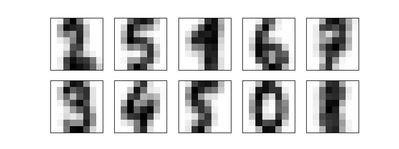

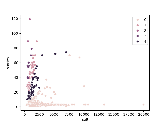
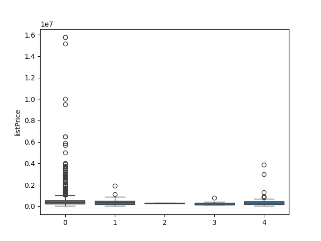
The example below also uses the K-Means clustering method to the Real Estate Data Chicago dataset. It applies the sqft (i.e., square), stories, and listPrice (i.e., price) features.

import pandas as pd
from sklearn.model_selection import train_test_split
import seaborn as sns
import matplotlib.pyplot as plt
from sklearn import preprocessing
from sklearn.cluster import KMeans
from sklearn.metrics import silhouette_score

# Loading the dataset
dataset = pd.read_csv('real_estate.csv', usecols = ['sqft', 'stories', 'listPrice'])
print(dataset.head())

# Cleaning the data (removing the rows with NaN)
dataset = dataset.dropna()

# Setting up training and test splits
data_train, data_test, target_train, target_test = train_test_split(dataset[['sqft', 'stories']], dataset[['listPrice']], test_size = 0.2, random_state = 0)

# Visualizing the data
sns.scatterplot(data = dataset, x = 'sqft', y = 'stories', hue = 'listPrice')
plt.savefig("data.png")

# Normalizing the data
data_train_norm = preprocessing.normalize(data_train)
data_test_norm = preprocessing.normalize(data_test)

# Fitting and evaluating the model
model = KMeans(n_clusters = 5, random_state = 0, n_init = 'auto')
model.fit(data_train_norm)

# Displaying the data fitted by the clustering algorithm
plt.clf()
sns.scatterplot(data = data_train, x = 'sqft', y = 'stories', hue = model.labels_)
plt.savefig("fitted_data.png")

# Displaying the distribution of prices in the clusters
plt.clf()
sns.boxplot(x = model.labels_, y = target_train['listPrice'])
plt.savefig("cluster_price.png")

# Displaying the Silhouette score for the algorithm’s performance evaluation
print(silhouette_score(data_train_norm, model.labels_, metric = 'euclidean'))

# Choosing the best number of clusters
clusters_num = range(2, 11)
fits = []
score = []

for cluster_id in clusters_num:
  # Training the model for the current value of cluster_id
  model = KMeans(n_clusters = cluster_id, random_state = 0, n_init = 'auto')
  model.fit_predict(data_train_norm)

  # Appending the model to the fits list
  fits.append(model)

  # Appending the Silhouette score to the scores list
  score.append(silhouette_score(data_train_norm, model.labels_, metric = 'euclidean'))

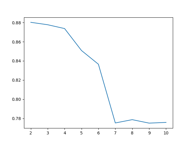
# Displaying the Silhouette scores obtained for different numbers of clusters
plt.clf()
sns.lineplot(x = clusters_num, y = score)
plt.savefig("score.png")

Output

Data:
      sqft  stories  listPrice
0  3000.0      2.0   750000.0
1  2900.0      2.0   499900.0
2  1170.0      2.0   325600.0
3  2511.0      2.0   620000.0
4  2870.0      3.0   850000.0
5  2800.0      2.0   599000.0
6  4200.0      2.0  1500000.0
7  1637.0      2.0   110000.0
8  2600.0      1.0   599990.0
9  3150.0      2.0   399900.0

Score: 0.8508240261996011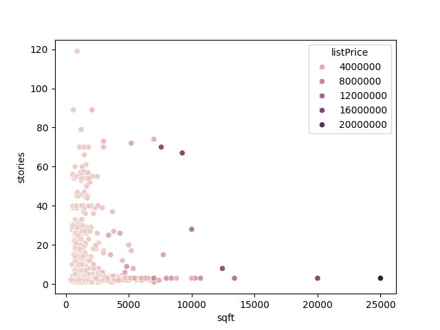

The Real Estate Data Chicago dataset (‘real_estate.csv’) can be download via the link below:

https://www.kaggle.com/datasets/kanchana1990/real-estate-data-chicago-2024

References

1. Hackeling, G. (2017). Mastering Machine Learning with scikit-learn, 2nd Edition. Packt Publishing Ltd.
2. Géron, A. (2019). Hands-On Machine Learning with Scikit-Learn, Keras, and TensorFlow, 2nd Edition. O’Reilly Media, Inc.
3. Tutorials Point. Scikit Learn Tutorial. Retrieved November 20, 2025, from https://www.tutorialspoint.com/.